Some people are suggesting that the averaged value I was using in the video continually
decreases due to floating point math precision, but I don't see how that could be.
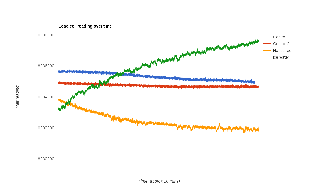
Here are some 10 minute runs where I just read the raw value from the load cell with no other math involved.
The runs were done in the order they appear in the chart legend.
Each run starts about 10 seconds after the last one, so you can see for example run 2 starts at about the value where run 1 finished.
In the last two runs I placed a hot/cold object near the load cell, about 1mm from the center of the bar.
I'm not really sure why there is such a quick change between the end of run 2 and the start of run 3, and also between runs 3 and 4.
It really does look like it's just a temperature related fluctuation.
The total reading fluctuation between hot coffee and ice water is about 6000, and for my load cell the difference
in reading for 100g was around 40000.
This means that I would get an error of about 15g if the temperature of the load cell changed from one of these extremes to the other
between calibration time and measurement time.
A temperature change of that magnitude in that time span seems quite unlikely, but we should keep in mind that the wind generated by the
motor running will cool the load cell somewhat.
I think if calibration is done immediately prior to each test run, and the total time the motor runs is kept short then the cooling of the
load cell during the test run will be negligible.
*** UPDATE 19 Mar 2017
I have to admit that the floating point truncation does cause the averaged value to change, as demonstrated by this sample program
provided by Jess Stuart in the comments.
#include <stdio.h>
#include <time.h>

int main(void)
{
  int cell=8000000;
  float count=0,fval;
  while(1){
    count=count+1;
    fval = ((count-1)/count)*fval + (1/count)*cell;
    printf("%d\n",(int)fval);
  }
  return 0;
}
However, this value is not limited to a decrease in the result, and it causes the output to change in discrete jumps rather than the smooth steady downward change seen in the video.
Here is a graph of the first thirty minutes (assuming 10 samples per second) of deviation from the input value. In this case the input value is 8000000, but note also that results will vary depending on the input
value, and some input values (eg. 1) cause no deviation at all.
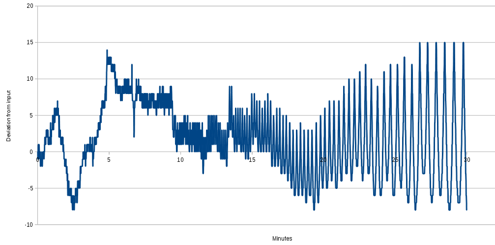
For this time frame at least, the deviation due to floating point truncation remains close to the true value, and is actually positive more than it is negative.
The first thing to note is how negligible this is when compared to the noise in the reading itself. If we plotted this on the above graph in the same scale, it would barely be even one pixel high.
In the video I was mostly running the sketch for less than two minutes, over which time the deviation is mostly positive, and only goes to -2 at greatest negative.
Anyway, the point is that the method of averaging that I used in the video is not a good one in the long term, and it's better to use a moving average like Jess suggests.
I am of course using a moving average in reall applications (eg. my thrust test stand) but I thought explaining that would add a bit too much to what I wanted to be a simple intro video to load cells.
For those who are wondering, here are the first half-million values of that graph above, showing why you don't want to use my method for a long-running application. Although the result values
still remain in the vicinity of the true value, there are increasingly wide swings to each side. Keep in mind this graph represents about 14 hours of sampling at 10Hz, so if you're just doing some quick testing over spans of a few minutes you can probably get away without using a proper moving average.
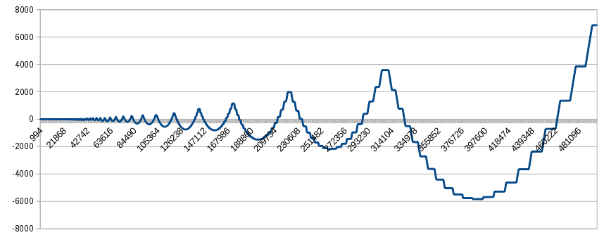
Comparing the first graph above with this graph at the same vertical scale, it looks like the deviation due to floating point truncation will become more significant than sensor noise after about 75 minutes.